This first experiment is called the three-polarizer paradox. It's not a true paradox—quantum mechanics predicts the result exactly—but the outcome is surprising enough to challenge our classical intuition. Place two polarizers at $90^\circ$ to each other: no light passes. Now insert a third polarizer at $45^\circ$ between them: suddenly $12.5\%$ of the light passes through. How can adding a filter increase transmission?To resolve the paradox, we will apply the ideas covered in the Introduction—states as kets, evolution via linear operators, and the Born rule for measurement outcomes—to a concrete physical property, the polarization of light.
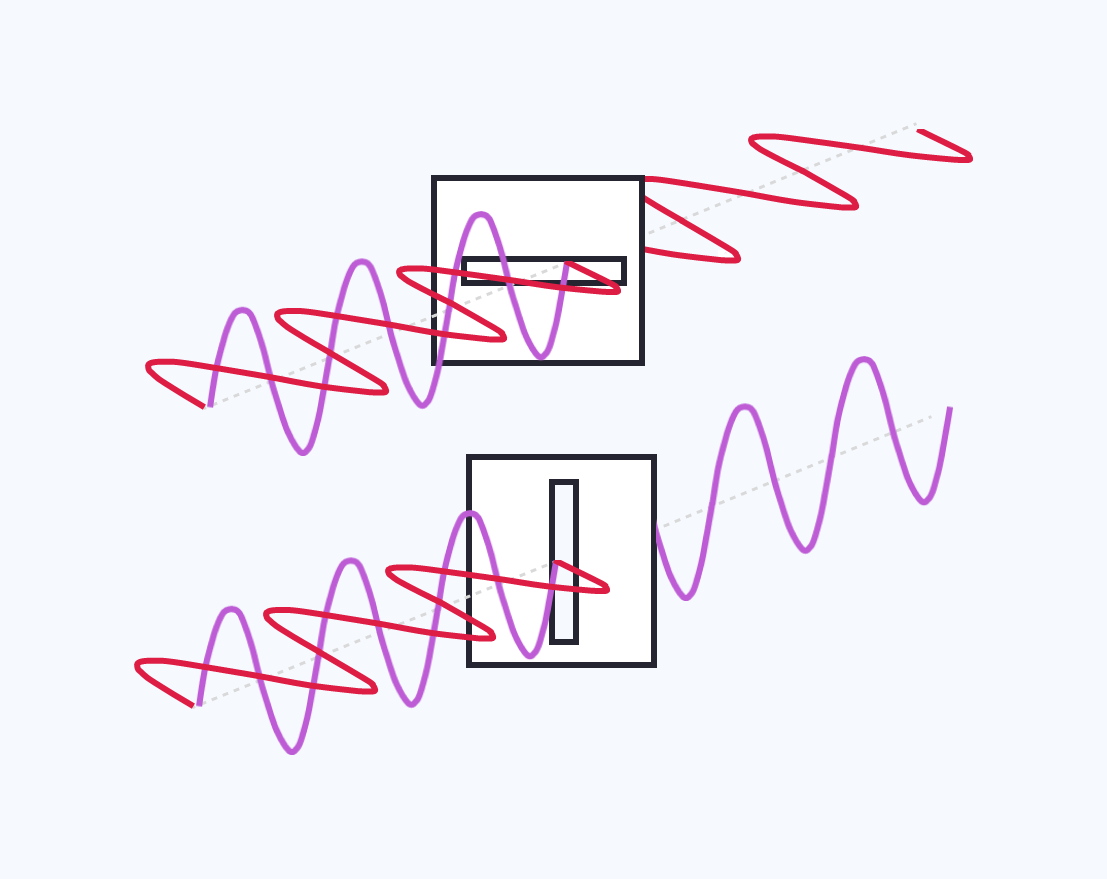
As light propagates, its electric field oscillates perpendicular to the direction of travel. The axis of this oscillation is the light's polarization. A photon can be polarized vertically, horizontally, or at any angle in between.
In the language of quantum mechanics, polarization is a quantum property described by a state vector. Two natural basis states are:
These states are orthogonal—a detector can distinguish them with certainty. But a photon can also exist in a superposition, such as the diagonal polarization:
This is exactly the kind of linear combination we studied in the Introduction.
.png)
A polarizer is an optical device that transmits light polarized along its axis and blocks light polarized perpendicular to it. Mathematically, a polarizer acts as a linear operator on the photon's quantum state—much like the transformation $R_{45}$ from the Introduction, but with a key difference: polarizers can lose photons.
The transmission probability follows from the amplitudes:
- If the photon's polarization is aligned with the polarizer (e.g., both horizontal), it passes with probability 1.
- If perpendicular (one vertical, one horizontal), it passes with probability 0.
- At 45° misalignment, the probability is $\cos^2(45°) = \frac{1}{2}$.
Crucially, the photon that emerges is now polarized along the polarizer's axis—the polarizer has changed the quantum state, not merely filtered it.
Explore how light behaves under different polarizer configurations. The simulation starts with a diagonally polarized laser beam (45°). Use the control panel to add polarizers and drag the pink dot to adjust their orientation. The percentage on the right shows how much light reaches the detector relative to the original beam: 100% means nothing is blocked, 0% means complete darkness.
Here is the puzzle:
- Place a horizontal polarizer followed by a vertical polarizer. Result: 0% transmission. Their axes are 90° apart, so the second blocks everything from the first.
- Now insert a 45° polarizer between them. Result: 12.5% transmission.
Adding a third filter lets light through. This defies classical intuition—more obstacles should mean less transmission, not more. Are we somehow creating photons?
We'll derive the 12.5% result exactly in the Quantum Predictions for the 3-Polarizers Paradox, using the operator formalism. The resolution lies in how polarizers transform quantum states—but first, let's confirm this effect is real.For more on the 3-polarizer paradox, have a look at this brief video:

We set up the experiment in a laboratory and measured the light intensity at the detector. The gist of the data is represented in the below table, which displays how the transmitted light intensity changes depending on the number and orientation of the polarizers.
This table was made using the data we collected in the lab. The column "lab result'' is the number of photons detected in the center of the beam (which gives the highest number of photons). The intensity is a comparison with the initial beam. We always considered the initial beam (with no optical devices) to be 100%.
The first line is then the result with nothing in the way of the laser. The next four values are measured with 1 polarizer, placed at different angles compared to the initial beam. We see the number of photons change for all four angles. Because the incident beam is at 45 degrees, all the photons pass.
We consider this value to be 100%. At -45 degrees, no photon should be able to pass. But, we can still detect some photons, which can come from different sources in the lab, any light coming from an instrument or misread on the detector. We place its relative value at 0%.
Curious of what an entanglement optical setup looks like? Here is a few picture of what we have:


Here is the representation of the setup you see in the picture. All of the equipment is shown, but the scaling is not representative.

On the left side, the laser emits a beam of photons. We then place a polarizing beam splitter to rotate the polarization of the beam at 45 degrees. Depending of the orientation of the beam splitter, you might not get 45 degrees, so you can add a half-wave plate to rotate it in the orientation you want: 45 degrees for us. Then, a set of lenses can be use to concentrate the beam in the detector. The beam is now set to pass through all the polarizers we want. We tested with 0, 1, 2 and 3 polarizers. Finally, on the right-side, the detector is placed at the center of the beam.
You can download all our data here:
The pattern is created by moving the detector one side of the laser beam, to the other. At each step of the detetor, we count the number of photons captured in the time allowed (generally 1 or 2 seconds).
All of the acquisition can be found in those csv. They all have 3 columns: the position of the detector, the angle of the polarizers and the number of photons detected.
Quantum mechanics describes what happens to individual photons when they pass through an optical set-up like the one described above.
The key property of photons to be described here is the polarization of photon.
Earlier we introduced the horizontal and vertical polarization states, $\ket{\leftrightarrow}$ and $\ket{\updownarrow}$, and the diagonal state $\ket{\diag}$. To complete our toolkit, we introduce the \emph{anti-diagonal} polarization:
The states $\ket{\diag}$ and $\ket{\adiag}$ form an alternative orthogonal basis—just as valid as $\{\ket{\leftrightarrow}, \ket{\updownarrow}\}$. We will need this basis in Part~3 when computing the action of a diagonal polarizer.
The quantum state of the photon evolves when light passes through a polarizer. A horizontal polarizer, denoted as \( P_{\leftrightarrow} \), allows horizontally polarized photons to pass through, and it absorbs or reflects the vertically polarized photons. When the polarizer absorbs or reflects a photon, the photon is basically lost. Thus, the evolution of a photon passing through a horizontal polarizer is as follows:
In other words, when the evolution operator \( P_{\leftrightarrow} \) acts on the state, it returns the state $\ket{\leftrightarrow}$; and when it acts on the state $\ket{\updownarrow}$, it returns \( \ket{\text{lost}} \).
The term~\( \ket{\text{lost}} \) does not represent a polarization state, but rather the state of the photon's availability. It indicates that the photon won't interact with our detector because it has been absorbed or reflected by the polarizer.
We keep track of these lost photons by defining a state called \( \ket{\text{lost}} \). This maintains a complete mathematical description and keeps the overall state normalized. We bear in mind, however, that a photon in the \(\ket{\text{lost}} \) state will not be used in any further calculations: the photon has effectively been \emph{lost}.
Similarly, a vertical polarizer applied to a vertically polarized photon lets it through, or mathematically, $P_{\updownarrow} \ket{\updownarrow} = \ket{\updownarrow}$. And a vertical polarizer applied to a horizontally polarized photon gets it lost, $P_{\updownarrow} \ket{\leftrightarrow} = \ket{\text{lost}}$.
We have carefully specified what happens to horizontally and vertically polarized photons when they go through filters.
But what happens to a diagonally polarized photon, like $\ket{\diag}$, when it passes through a horizontal filter?
Recalling the evolution of quantum states in the Introduction, we use the linearity property of the evolution operator $P_\leftrightarrow$:
If this is the quantum state of the photon that reaches the detector, we can calculate the probability that the photon hits the detector. It's the probability that the photon is not lost, or in other words, it's the probability that a measurement of $\{\ket{\leftrightarrow},\, \ket{\text{lost}} \}$ returns $\ket{\leftrightarrow}$. This probability is given by the square of the amplitude pertaining to the component~$\ket{\leftrightarrow}$ in the expression above.
The intensity of a beam of light is proportional to the number of photons in that beam: the more photons, the more intense the light is.
If we send a beam of light, composed of multiple photons, and if each photon has a 50% chance of passing through, then the intensity of the outgoing beam shall be half that of the incoming beam.
In general, the intensity of the measured beam ($I$) is equal to the probability of measuring a single photon multiplied by the intensity of the incoming beam:
We are now equipped to compute what quantum theory predicts in various scenarios. In four parts, we will study the optical set up with no polarizer, one, two and then three polarizers.
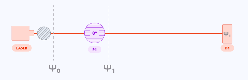
Let us consider first the simplest scenario, where a prepared photon propagates freely to the detector without encountering any polarizers. (In fact, because we wanted to prepare diagonally polarized photons, we inserted a diagonal filter right at the laser; but this simply amounts to a laser that emits diagonaly polarized photon.) See the below figure.
.png)
After the photon exits the laser (and the diagonal polarizer), it is prepared in a diagonal state of polarization:
No polarizer affects the photon, so it propagates freely to the right end of the optical table.
Since no component of its quantum state is lost, it will be detected regardless of its polarization state.
The measured intensity is, therefore, the whole of the incoming intensity:
In this scenario, we have added a horizontal polarizer between the locations of preparation and detection, see the below figure. This scenario corresponds to what we have studied in the previous section.
The initial state is given by
The state $\ket{\psi_1}$ can be computed by applying the horizontal polarizer, $P_{\leftrightarrow}$, as we did before:
The intensity at the detector is, as we have seen previously,
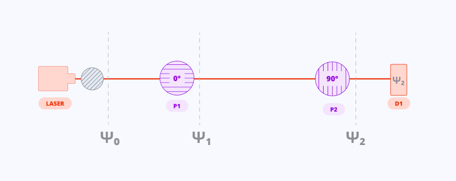
We now consider the insertion of a vertical polarizer as depicted in the above figure.
Again, the initial state is given by $\ket{\psi_0} = \ket{\diag}$.
Applying the first (horizontal) polarizer, we obtain
where $\ket{\text{lost}_{P_1}}$ denotes a state for the photon where it has been lost at the first polarizer.
Applying the second (vertical) polarizer, we find
The probability of measuring a non-lost photon is $0$. Therefore, the intensity at the detector is
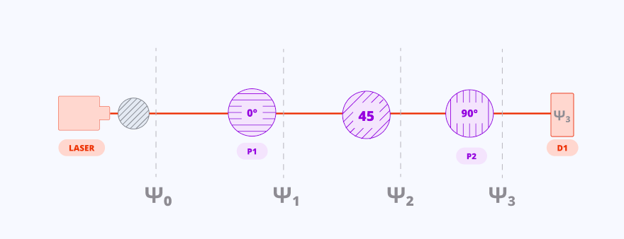
We now consider the final optical set-up, where a polarizer oriented at 45° is inserted between the horizontal and vertical polarizers. See the above figure.
As we have seen before, the initial state~$\ket{\psi_0} = \ket{\diag}$ evolves into $\ket{\psi_1} %&= P_{\leftrightarrow}\ket{\psi_0}\\
= \frac{1}{\sqrt{2}}\ket{\leftrightarrow} + \frac{1}{\sqrt{2}} \ket{\text{lost}_{P_1}}$.
Then, between time $t_1$ and $t_2$, a diagonal polarizer is applied:
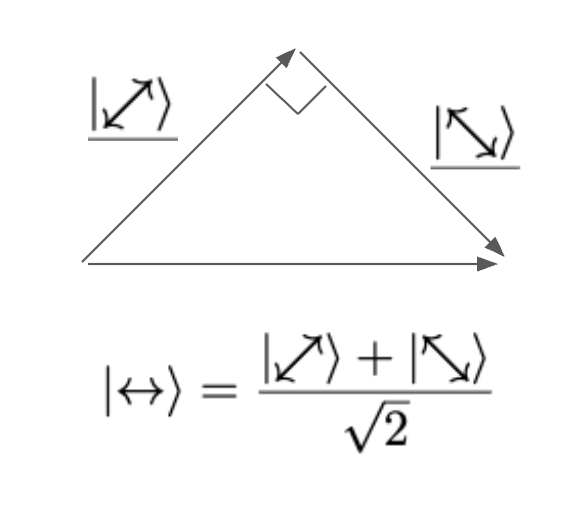
How do we carry on with this calculation? The second term is easy to compute: $P_{\diag}$ applied to a previously lost photon keeps the photon lost, so $ P_{\diag} \ket{\text{lost}_{P_1}} = \ket{\text{lost}_{P_1}}$. But how do we compute $P_{\diag} \ket{\leftrightarrow}$? The key is to express the state $\ket{\leftrightarrow}$ in terms of the vectors $\ket{\diag}$ and $\ket{\adiag}$. Consider what happens when we sum $\ket{\diag}$ and $\ket{\adiag}$:
The resulting state is not normalized, but by multiplying each side of the above equation by $\frac{1}{\sqrt 2}$, we obtain
By the same logic, subtracting the diagonal states gives the vertical state:
Applying $P_\diag$ to $\ket{\diag}$ leaves it as $\ket{\diag}$, while applying $P_\diag$ to $\ket{\adiag}$ makes the photon $\ket{\text{lost}}$. Therefore, going back to equation to our previous equation for $\ket{\psi_2}$ we have,
We then apply the third polarizer, $P_{\updownarrow}$:
The intensity at the detector is, therefore,
The “paradox” in this optical setup is the following: classically, inserting an additional filter should only make transmission less likely, not more. Yet here, adding a third polarizer—placed between two polarizers that completely block the light—allows some light to pass through.
The analysis resolves this puzzle. A polarizer does more than simply block or transmit light: it changes the polarization state of the photons that pass through it. As a result, the outgoing light is effectively rotated. In quantum mechanics, this behavior is described using the notion of states and their evolution, followed—only at the end—by a measurement rule that connects these states to observed intensities.
If you want to see the three polarizer paradox from your own eyes, here are some Youtube videos we found to be accurate and insightful!


