In Experiment 1, we explored how polarizers transform the polarization state of photons—and saw that quantum mechanics predicts results that defy classical intuition. Now we turn to another quantum degree of freedom: the photon's path.
The double-slit experiment is perhaps the most iconic demonstration in quantum mechanics. Here is the puzzle: send photons through two slits, one at a time, and record where each one lands on a detector screen.
Each photon arrives as a single localized dot—clearly particle-like. But after thousands of photons, the collection of recorded dots forms an interference pattern—the kind of pattern we associate with waves.Where does the interference come from, if each photon travels alone?
The answer lies in superposition. Just as a photon's polarization can be a superposition of $\ket{\updownarrow}$ and $\ket{\leftrightarrow}$, a photon's path can be a superposition of $\ket{A}$ and $\ket{B}$—passing through both slits simultaneously. The interference pattern emerges from how these path amplitudes combine, exactly as the Introduction described for any quantum superposition.
Explore how the interference pattern depends on the geometry. The simulation lets you adjust:
- Number of slits ($N$)
- Slit width ($w$)
- Slit separation ($d$)
- Wavelength ($\lambda$)
Drag the pink dots on the control panel and observe how each parameter affects the pattern. Pay attention to what happens when you cover one slit—the fringes disappear, leaving only the wide envelope.
The prove you that the animation is not lying, we built the setup in a lab.
This is the data we got from our lab setup. The left plot has two curves, for either slit covered. In the following section, we will explain what we did in the lab, what the data shows, what the explanation is for all of this and the maths behind the theoretical curves.
Curious of what an optical setup looks like? Here are some pictures of the double slit and the single slit setup (same setup, we just change the slit).


The diagram below represents the double-slit setup shown in the previous pictures. While all key components are included, the scaling is not to size.

We use a laser with a wavelength of 808 nm as the light source. The beam first passes through a half-wave plate and a beam splitter, which together ensure that its polarization is diagonal—an important detail for certain interference effects.
The beam is then focused by a lens onto the double slit (or single slit), after which it continues toward the detector.
Our detector is a single-photon counting module mounted on a motorized linear translation stage, allowing it to scan across the interference pattern and build up a full spatial intensity profile over time. In front of the detector, we place a set of optical filters, including long-pass filters, to prevent saturation and reduce background noise. These detectors are extremely sensitive and can handle a maximum of about 250,000 photons per second—meaning even ambient light must be carefully controlled.
For the single-slit measurements, we used the same double-slit mask with one of the slits covered, allowing us to isolate the contribution of each slit individually. A dedicated single slit could also be used, but covering one slit allows for direct comparison under otherwise identical conditions. Our approach allows us to observe the contribution of each individual slit and clearly visualize the spacing between them in the resulting graph.
You can download all our data here:
The files have 3 columns. The first one is the distance travelled by the actuator in $\mu$m. The second column is the number of counts seen by the detector, in a range of 2 seconds. The last column is the same number of counts, but per seconds.


In the first plot, two curves are displayed–each corresponding to the intensity with one of the slits covered.
In the second plot, we can clearly distinguish three main peaks, indicating the presence of interference. The number and size of the peaks are determined by the geometry of the double slit—depending on the slit width and spacing, you might observe three, four, five, or more peaks. To anticipate the number and structure of the peaks, you can refer to the interactive animation provided at the beginning of the experiment.
Typically, the central peak is the most intense, and the adjacent peaks should have roughly equal intensity. If they do not, it may indicate that the slits are not perfectly aligned perpendicular to the incoming beam. The horizontal distance between the two individual curves is approximately 175 $\mu m$, which corresponds closely to the actual slit separation of about 200 $\mu m$.
As a final check, we compare the experimental data with theoretical predictions using the equations from the theory section. The theoretical curve, shown as a gray dashed line, matches the general pattern, although we observe slight deviations in intensity and width. These discrepancies can be attributed to minor misalignments in lens placement or imperfections in the linear actuator’s motion.
A first surprising effect to be explained is that when coming through a narrow slit, the beam of photons does not get narrow. Quite the opposite: it widens up. This phenomenon is called diffraction.
The easiest way to understand, at a high level, why a particle diffracts when it passes through a slit is by invoking Heisenberg's uncertainty principle. Here's what the principle says:
- A particle's position and momentum cannot both be precisely defined at the same time.
- The more precisely position is constrained, the more uncertain momentum becomes, and vice versa.
When a photon passes through a slit of a certain width, we know its position along the vertical axis (the slit fixes it within that range). This means that the uncertainty in its vertical momentum must increase, following Heisenberg's uncertainty principle.
That uncertainty in momentum translates into a spread of possible directions the photon can take once it has passed the slit. Instead of traveling in a perfectly straight line, its sideways momentum has a significant spread. So instead of having one exact momentum value pointing straight ahead, the photon now has many possible sideways momentum values, each value tied to a certain probability. The result is that many possible shifted directions are realized, with different probabilities, forming what we observe as a diffraction pattern.
To put it simply:
- Narrow slit $\rightarrow$ small uncertainty in position $\rightarrow$ large uncertainty in momentum $\rightarrow$ wide diffraction pattern.
- Wide slit $\rightarrow$ large uncertainty in position $\rightarrow$ small uncertainty in momentum $\rightarrow$ narrow diffraction pattern.
The mathematical form of this diffraction pattern is:
This formula will reappear throughout subsequent experiments.
Heisenberg's uncertainty principle is very general, it doesn't just apply to position and momentum, but also to other pairs of quantum properties. More broadly, this is called quantum complementarity.
Take polarization, for example. A photon can be in the state $\ket{\updownarrow}$, for instance. If we then measure it along the vertical-horizontal axes, we will get a definite outcome: it will appear vertical.
But what if we measure it along the diagonal ($\ket{\diag}$ and $\ket{\adiag}$) axes? In that case the outcome is no longer certain. We can in fact write the $\ket{\updownarrow}$ state as a superposition of the diagonal states:
What the above equation means is that if we test the $\ket{\updownarrow}$ state with a diagonal polarizer, it has a 50 percent chance of coming out one way, and a 50 percent chance of coming out the other way. The core idea here is that no photon can be perfectly defined in both descriptions, meaning vertical and diagonal at the same time.
We have seen that when a system is in superposition, its state is expressed as a sum of many other states, each of which is multiplied by an amplitude. These amplitudes correspond to a complex number, and so it can be decomposed into a modulus and a phase.
We can think of a phase as a point rotating on a circle. Mathematically, it's represented by a complex exponential:
In the above equation, $i$ is the imaginary number, $k = 2\pi/\lambda$ is the wave number, and $s$ is the distance the photon has traveled.
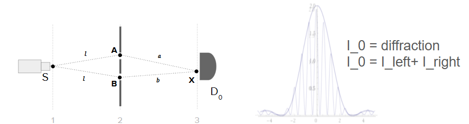
Using Dirac notation, we can describe the photon's journey mathematically. At the source, the state is $\ket{\psi_0} = \ket{S}$. After passing through the double slit, the photon is in a superposition of both paths:
Here, the factor $1/\sqrt{2}$ ensures normalization. As each path accumulates phase based on distance traveled, interference emerges. The full derivation appears in the Mathematical Derivation section below.
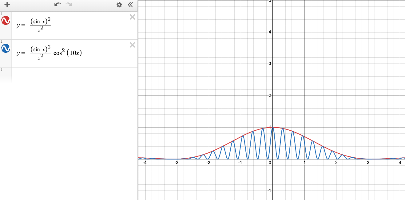
The equation that describes the diffraction pattern of a photon passing through a single slit is:
Here, $w$ represents the width of the slit, $\theta$ is the angle between a point on the screen and the center of the slit, and $\lambda$ is the wavelength of the photons. On the right, we can see an example of a diffraction pattern.

In this experiment, the polarization of the photon does not matter, we only track its position. The photon starts at the source in the state:
As the photon propagates toward the slits, its wavefunction overlaps with both slits, as well as the opaque parts of the mask (the area between/around the slits, which blocks or absorbs photons). Some photons hit the mask and are absorbed (lost), while others pass through slit A or slit B. Let $A_{\text{pass}}$ represent the amplitude of a photon that successfully passes through a slit, and $A_{\text{lost}}$ the amplitude of a photon that is absorbed.
Since we cannot easily predict the number of lost photons and because they do not contribute to the interference pattern, we drop the $\ket{\text{lost}}$ term. The state becomes:
The photon then propagates to the detection screen. Consider a specific point on the screen, $\ket{y}$. If $\ket{y}$ is at the center, the distances from A and B are equal. If $\ket{y}$ is above or below the center, the path lengths differ. Let “a” be the distance from slit A to $\ket{y}$, and “b” the distance from slit B to $\ket{y}$. At that position, the amplitudes from both slits combine:
For a screen at distance $L$ from slits separated by $d$, the path difference in the small-angle regime ($y \ll L$) is:
where $\theta$ is the angle from the optical axis. We use this approximation throughout.
.png)
As the photon propagates from each slit to position $y$, each path acquires a phase proportional to the distance traveled:
The full state now includes contributions at every screen position. Focusing on a single position $y$:
(The "$\cdots$'' indicates similar terms for other positions $y'$ on the screen.)
To compute the probability of detecting a photon at $\ket{y}$, we square the coefficient in front of $\ket{y}$. We define $I_0$ as the peak intensity at the center of the screen ($\theta = 0$), before any angular dependence is applied. With this definition, the interference term becomes:
This term oscillates between $0$ (destructive interference, when $b - a = (n + \tfrac{1}{2})\lambda$) and $2I_0$ (constructive interference, when $b - a = n\lambda$).
Finally, the interference term must be combined with the single-slit diffraction envelope. Each slit has finite width $w$, which causes the light to spread according to:
The complete intensity pattern combines both effects—interference fringes modulated by the diffraction envelope:
Here:
- $I_0$ is the intensity from a single slit at $\theta = 0$. With both slits open and constructive interference, the maximum intensity is $4I_0$, because intensity scales as amplitude squared (doubling amplitude quadruples intensity).
- $d$ is the slit separation (center to center)
- $w$ is the width of each slit
- The term $\left(1 + \cos(\cdots)\right)$ creates the interference fringes (ranges from 0 to 2)
- The term $\left(\frac{\sin \alpha}{\alpha}\right)^2$ is the diffraction envelope
Note: We replaced the path difference $(b-a)$ with its geometric equivalent $d \sin\theta$, valid in the far-field regime.
If you want to see the three polarizer paradox from your own eyes, here are some Youtube videos we found to be accurate and insightful!


