
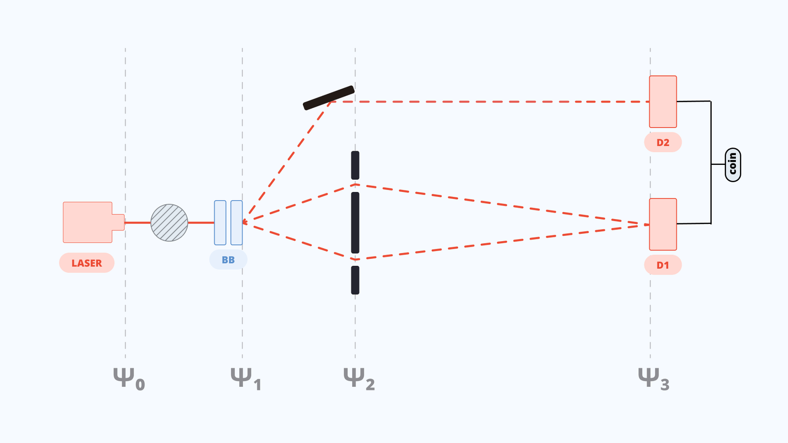
This section presents experiments 5.1-5.3, which set up the puzzle that the quantum eraser will resolve in experiment 6. Starting from the entanglement setup of experiment 4, we add a double slit and polarizers on the signal path. The detector $D_1$ is mounted on a linear actuator to scan the diffraction and interference patterns.
This section presents one of the most counterintuitive aspects of entanglement. If we reproduce the same experiment as experiment 3 (double slit with polarizers), but using entangled photon pairs instead of single photons, the results change completely.
We proceed step by step, adding one component at a time to observe how each affects the final pattern. For details on the entanglement source and BBO crystal, refer to experiment 4. The development is split into three parts:
- 5.1: Double slit only. We observe interference.
- 5.2: Orthogonal polarizers on each slit. Interference disappears due to which-path information.
- 5.3: A third polarizer at $45^\circ$. Surprisingly, interference does not return.
The key puzzle: in Experiment 3, the third polarizer restored interference by erasing which-path information. With entangled photons, it fails. The which-path information is no longer stored in the signal photon's polarization. Instead, it is encoded in the idler photon. No local operation on the signal path can erase it. Try the animation first, then examine the results below.
We start with the same setup as in Experiment 4, but remove the two polarizers in front of the detectors (they were only needed to verify the polarization state). Detector $D_1$ is mounted on a linear actuator to scan the full pattern.


Both graphs show a clear interference pattern. The right graph has fewer counts because it records only coincidences: events where $D_1$ and $D_2$ both detect a photon within a 10 ns window.
As expected, a double slit produces interference.
The data is available here:
This file contains 6 columns:
- Polarizer angle 1 (not applicable here)
- Polarizer angle 2 (not applicable here)
- Actuator position
- Sweep number
- Counts at $D_1$
- Counts at $D_2$
- Coincidences between $D_1$ and $D_2$
All counts are recorded over 20-second windows.
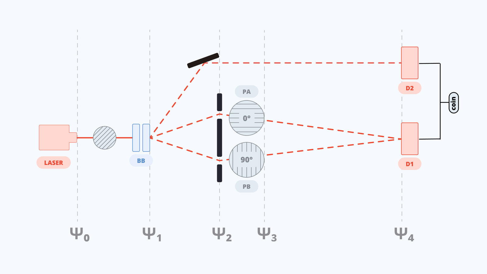
We place a vertical polarizer ($P_A$ at $0^\circ$) in front of slit $A$ and a horizontal polarizer ($P_B$ at $90^\circ$) in front of slit $B$. This encodes which-path information in the polarization.


Interference has disappeared. As in Experiment~3, orthogonal polarizers on each slit make the paths distinguishable, destroying interference. We observe only diffraction (the sum of two single-slit patterns).
The count rate also drops significantly because each polarizer blocks half the photons.
You can download the data here:
Column format is identical to Exp 5.1.
All counts are recorded over 20-second windows.
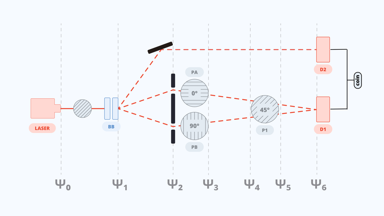
We now add a third polarizer at $45^\circ$ after the double slit, just as we did in Experiment 3.


This result is surprising. In Experiment 3 (with non-entangled photons), the $45^\circ$ polarizer restored interference by erasing which-path information. Here, with entangled photons, interference does not return.
By "losing interference", we mean that each slit acts as an independent single slit. The observed pattern is the sum of two diffraction envelopes, with no oscillating fringes.
You can download the data here:
Column format is identical to previous experiments. The first two columns (polarizer angles) can be ignored for $P_2$. All counts are recorded over 20-second windows.
In this experiment, entangled photon pairs pass through a double slit with no polarizers. We track both polarization and position.
Step 1. Initial entangled state.
The BBO crystal produces polarization-entangled pairs in the Bell state $\ket{\Phi^+}$. Using subscript 1 for the signal photon and 2 for the idler:
The signal photon travels toward the double slit. The idler travels directly to detector $D_2$.
Step 2. Signal photon at the double slit.
The signal photon can pass through slit $A$ or slit $B$, entering a spatial superposition. The full state (polarization $\otimes$ signal position $\otimes$ idler position) is:
Here $\ket{A}_1$ and $\ket{B}_1$ denote the signal photon's position at slit $A$ or $B$, and $\ket{S}_2$ is the idler's position (traveling toward $D_2$). The symbol $\otimes$ just means "and", we're combining polarization and position into one complete description.
Step 3. Propagation to detectors.
The signal photon propagates from each slit to position $y$ on the detection screen. The path lengths differ: distance $a$ from slit $A$, distance $b$ from slit $B$. Each path acquires a phase factor:
The idler propagates distance $m$ to detector $D_2$:
After the propagation on the screen, the full state is decomposed as a sum of various terms at different locations. Making explicit one such location, the state becomes:
Step 4. Detection probability at $D_1$.
To find the probability of detecting the signal photon at position $y$, we compute the squared amplitude. The key observation: both polarization terms ($\ket{\updownarrow\updownarrow}$ and $\ket{\leftrightarrow\leftrightarrow}$) have identical spatial amplitudes. The polarization does not encode any which-path information.
The path lengths $a$ and $b$ depend on the detection position $y$. Using the path-difference geometry from experiment 2:
The spatial amplitude is:
The intensity (proportional to the squared amplitude) is:
This is the standard double-slit interference pattern:
The intensity oscillates between 0 (destructive interference) and a maximum of 2 (constructive interference), with fringe spacing $\Delta y = \lambda L / d$. We omit the single-slit diffraction envelope here for clarity.
Interpretation.
Without polarizers at the slits, the paths remain indistinguishable. Both polarization components ($\ket{\updownarrow\updownarrow}$ and $\ket{\leftrightarrow\leftrightarrow}$) traverse both slits with identical amplitudes. The entanglement does not destroy interference because no which-path information is encoded anywhere.
This matches our experimental observation: clear interference fringes in both singles and coincidences.
We place a vertical polarizer ($0^\circ$) in front of slit $A$ and a horizontal polarizer ($90^\circ$) in front of slit $B$. This encodes which-path information in the polarization.
Step 1. Initial entangled state.
As before, the BBO produces the Bell state:
Before the polarizers, the signal photon is in a spatial superposition of both slits:
Step 2. Polarizer filtering.
The polarizers act as filters, not state assigners. Each polarizer transmits only the matching polarization component:
- Vertical polarizer at $A$: transmits $\ket{\updownarrow}_1$, blocks $\ket{\leftrightarrow}_1$
- Horizontal polarizer at $B$: transmits $\ket{\leftrightarrow}_1$, blocks $\ket{\updownarrow}_1$
Expanding the state before filtering:
After filtering, the blocked components are absorbed:
The $\ket{\text{lost}}$ term represents photons blocked by the polarizers—half the total. Since these do not reach the detector, we drop them from subsequent analysis:
Step 3. The key insight: which-path information.
Look carefully at the surviving state. The polarization is now perfectly correlated with the slit:
- $\ket{\updownarrow}_1\ket{\updownarrow}_2\ket{A}_1$: signal is vertical, idler is vertical, path is slit $A$
- $\ket{\leftrightarrow}_1\ket{\leftrightarrow}_2\ket{B}_1$: signal is horizontal, idler is horizontal, path is slit $B$
The idler photon's polarization now reveals which slit the signal photon passed through:
This is which-path information, encoded in the entangled partner.
Step 4. Propagation to detector.
The signal photon propagates to position $y$ on the screen, with path lengths $a$ (from slit $A$) and $b$ (from slit $B$):
Step 5. Detection intensity.
To find the intensity at position $y$, we compute the squared amplitude. The key observation: the two terms correspond to orthogonal polarization states of the idler ($\ket{\updownarrow}_2$ vs. $\ket{\leftrightarrow}_2$).
Orthogonal states cannot combine—they remain distinct contributions that add independently. This means the phases $e^{ika}$ and $e^{ikb}$ never add or cancel. Each term contributes its own intensity:
The intensity is independent of position $y$:
There are no oscillating fringes. The observed pattern is the sum of two single-slit diffraction envelopes.
Interpretation.
The polarizers have tagged each path with a distinct polarization, and because the photons are entangled, this tagging is mirrored in the idler:
The idler states $\ket{\updownarrow}_2$ and $\ket{\leftrightarrow}_2$ are orthogonal, so these two terms in the wavefunction cannot recombine. The phases $e^{ika}$ and $e^{ikb}$ contribute independently, they never add constructively or cancel destructively. This is the physical origin of the lost interference.
Compare to experiment 3 (non-entangled photons): there, the which-path information was stored only in the signal photon's polarization, and a $45^\circ$ polarizer could erase it. Here, the distinguishing property is in the idler, beyond our reach on the signal path.
We now add a $45^\circ$ polarizer after the double slit, just as we did in Experiment~3. With non-entangled photons, this restored interference. Will it work here?
Step 1. State after the slit polarizers.
From Exp 5.2, after the orthogonal polarizers at the slits and propagation to position $y$:
The signal polarization is correlated with the path, and this correlation is mirrored in the idler.
Step 2. Applying the $45^\circ$ polarizer.
The $45^\circ$ (diagonal) polarizer projects both $\ket{\updownarrow}$ and $\ket{\leftrightarrow}$ onto $\ket{\diag}$, each with amplitude $\frac{1}{\sqrt{2}}$:
After the polarizer, the signal photon's polarization is $\ket{\diag}_1$ for both paths. The state becomes:
Step 3. Why interference still fails.
At first glance, the signal photon now has the same polarization $\ket{\diag}_1$ regardless of which slit it passed through. In Experiment 3, this was enough to restore interference.
But look at the full state. The two amplitudes are:
The signal polarizations are now identical. But the idler polarizations are still orthogonal: $\ket{\updownarrow}_2$ and $\ket{\leftrightarrow}_2$ are perpendicular states that cannot combine.
Step 4. Computing the detection intensity.
For interference to occur, the two path amplitudes must be indistinguishable in every degree of freedom. Here, they differ in the idler's polarization.
Because the idler states are orthogonal, the two terms contribute independently to the intensity. The phases $e^{ika}$ and $e^{ikb}$ never add or cancel—each term contributes its own intensity separately:
The cross-terms that would produce interference (containing $e^{i(ka-kb)}$ and $e^{-i(ka-kb)}$) vanish because they multiply orthogonal idler states.
Interpretation.
The $45^\circ$ polarizer erased the which-path information from the signal photon. But the information still exists in the idler photon:
- Idler is $\ket{\updownarrow}_2$ $\Rightarrow$ signal came through slit $A$
- Idler is $\ket{\leftrightarrow}_2$ $\Rightarrow$ signal came through slit $B$
No operation on the signal path alone can erase information stored in the idler. The which-path information has been "exported" to the entangled partner, where it remains intact.
This is the fundamental difference from Experiment 3: with non-entangled photons, all which-path information was local to the signal photon, so a local polarizer could erase it. With entangled photons, the information is also encoded in a remote system.
What would restore interference?
To recover interference, we would need to erase the which-path information from the idler as well. This can be done by measuring the idler in the diagonal basis and post-selecting on the result. This is the quantum eraser protocol, explored in the next experiment.


