Here, we explain how quantum mechanics works: the mathematical objects it uses, the predictions it makes, and how those predictions are tested experimentally.
Rather than beginning with rigorous formalism, we start in the middle — by offering simple statements that capture the core ideas. The downside of simplicity is that it can be inaccurate, but as you move through the website, we’ll gradually refine and deepen the presentation.
The upshot is that you can begin understanding quantum theory with only minimal mathematical background. For now, you only need vectors in 2 dimensions.
As is customary in physics, systems are described by their states. As the system evolves in time, the state evolves too, providing us with a state for each moment. Think of it like a movie: each frame shows the state of a particular scene at a specific instant. As the film runs, the frames change, and we see how the story evolves over time. The same applies to states in physics.
For instance, an apple may be in the state “red”, or “eaten”. These are its classical states — definite properties that describe the system and which we can measure. Consider the fridge of someone who enjoys red apples. The red apple may evolve to the state “eaten”, while the “eaten” apple remains “eaten”.
In quantum mechanics, systems are still described by states — but now they are quantum states.
A quantum apple can also be in one of two definite states: \( \ket{\text{red}} \), \( \ket{\text{eaten}} \) (don't worry about this special notation for now). But unlike a classical apple, a quantum apple doesn’t have to be in just one of these states. It can be in a superposition of being red and being eaten — a kind of combination of two equally real states. For example, the apple might be in the state:
The letter $\Psi$ ('Psi') is often used to denote the quantum state. We could have called it "A", "Some-Incredible-Name", or anything else. It's simply a convention to call it $\Psi$, no need to overthink it. The subscript ``0" serves to label the state at an initial time ($t=0$), it helps us see this is the initial state we're talking about. As we can see, $\Psi$, a quantum state, is made out of other states ($\ket{\text{red}}$ and $\ket{\text{eaten}}$).
The numbers~$\sqrt{\frac{2}{3}}$ and~$\frac{1}{\sqrt{3}}$ are called amplitudes. We will cover them in more detail later, but in the meantime, we can think of them as indications of how much of each state we're adding into the "mix" that is~$\Psi$, and as a result, how likely we are to find it. Sort of like weights for ingredients in a recipe.
Between time $0$ and time $1$, our quantum apple may evolve in the following way: the red apple rots, while the eaten apple remains eaten. Simple as that! Mathematically:
Therefore the quantum state of the apple at time $1$ would be:
Let's now make this more interesting. When it starts rotting, the red apple won't rot all at once. It will be a gradual process over time. At first, the apple is mostly red, with just a tiny chance of being rotten. But as time moves forward, the "red" part shrinks while the "rotten" part grows.
So instead of the apple flipping from red → rotten in one step, it gradually shifts, like this:
- At $t=0$: all red, no rotten yet.
- At $t=0.25$: mostly red, a little rotten.
- At $t=0.75$: almost all rotten, barely red.
- At $t=1$: fully rotten
But in the meantime, the “eaten” part, however, stays exactly as it was. So for example, the state could evolve step by step like this:
This is a simple model of how amplitudes can flow continuously between states. True physical processes, like radioactive decay, have a similar evolution. In a decay, a particle doesn’t just suddenly vanish, it gradually shifts from one state into another, with the mixture of states changing step by step.
Changes in quantum states are gradual, like the apple that smoothly flows from one state into another, via a superposition. As we are often interested in the state at some key moments, for instance at times $0$ and $1$, the gradual change accumulates into a discrete change.
This is a major difference with the classical picture, where our classical apple was described by either of the states "red", or "eaten". It was therefore evolving according to either
$$
\text{"red"} \mapsto \text{"rotten"} \, ~~~\text{or}~~~ \text{"eaten"} \mapsto \text{"eaten"}\,.
$$
On the other hand, our quantum apple is initially in a superposition of $\ket{\text{red}}$, and $\ket{\text{eaten}}$.
Therefore, between time $0$ and time $1$, the evolution of $\ket{\text{red}} \mapsto \ket{\text{rotten}}$, and $\ket{\text{eaten}} \mapsto \ket{\text{eaten}}$ happens in superposition.
After time $1$, suppose that we want to measure our quantum apple in order to determine if it is rotten or eaten. What should we expect?
This is like opening Schrödinger’s famous box with the cat inside, which is either alive or dead. Before we open the box, the apple’s state includes both “rotten” and “eaten” at once. But when we check, we only observe one of the two outcomes: either a rotten apple, or an eaten apple.
The measurement device (our eyes, or any detector) will register one definite result. Quantum mechanics doesn’t let us predict which one we will see, it only gives us probabilities. To find these probabilities, we simply square the amplitudes of the given states.
- The outcome "rotten" will be recorded with probability $\left( \sqrt{\frac{2}{3}}\right)^2 = \frac{2}{3}$;
- The outcome "eaten" will be recorded with probability $\left( \frac{1}{\sqrt 3}\right)^2= \frac{1}{3}$;
This is just like Schrödinger’s cat: the description includes multiple possibilities at once (the states in superposition), but our experience of opening the box always returns just one clear outcome.
The quantum apple is a good teaser to get a generic idea of quantum mechanics. The superposition of states, the evolution that also happens in superposition, and the seemingly probabilistic measurement has already been expressed.
But in order to dive deeper into quantum mechanics, we must be able to go into the more mathematically precise descriptions of quantum systems, and for that, understand the various tools that are used. What even is a ket, “$\ket ~$”? And why are we allowed to add them like we did the description of $\ket{\Psi_0}$? What about the amplitudes... can they be any number?
In this section, we address those questions by giving further details on what the mathematical objects are that are involved in quantum mechanics.
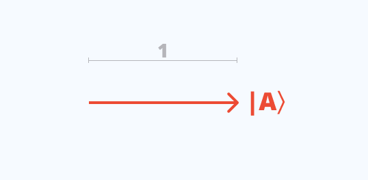
Quantum states are represented by vectors of unit length, namely, of length equal to 1. This is what a ket is: a vector of unit length.
Commonly, we write inside the ket a convenient label representing the state, such as $\ket{\text{red}}$ for the color red or $\ket A$ for a property labeled by $A$.
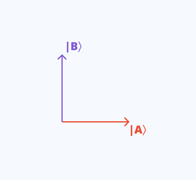
Two states, like $\ket A$ and $\ket B$ are distinguishable if it is possible to tell them apart with certainty, in which case they are then orthogonal. One can imagine orthogonality as two perpendicular arrows in 2D.
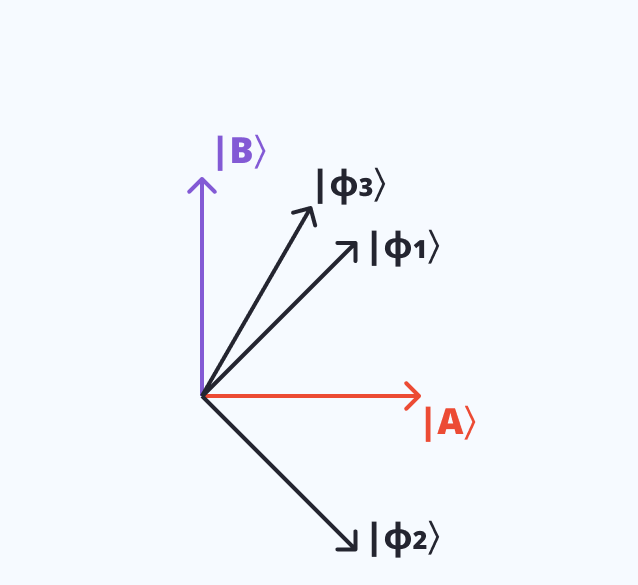
The superposition principle states that combinations of distinguishable states also form a valid quantum state, so long as the newly formed vector is also of unit length.
Thus, if $\ket A$ and $\ket B$ are valid orthogonal states, then by the superposition principle, all of the following states are also valid states:
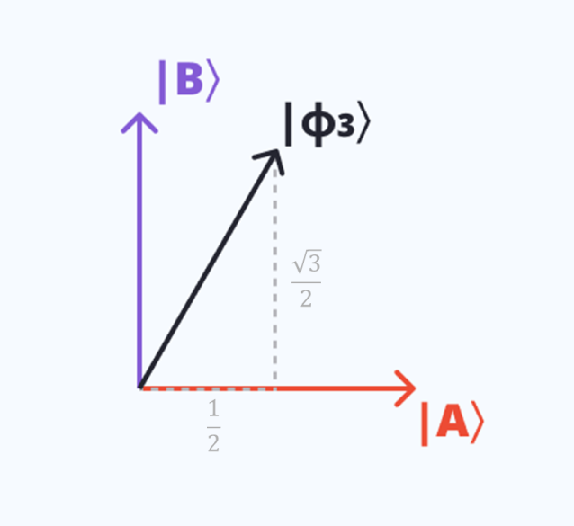
Let us verify that $\ket{\phi_3}$ is a vector of length one (also called a valid state, or a normalized state).
Geometrically, the length of $\ket{\phi_3}$ can be computed from the lengths of the horizontal and vertical projections.
The horizontal projection, or the projection onto $\ket A$, has length $\frac 12$; and the vertical projection onto $\ket B$, has length $\frac{\sqrt 3}{2}$.
Using Pythagoras's theorem, we find that the length of $\ket{\phi_3}$ is
Algebraically, we took the amplitudes, $\frac 12$ and~$\frac{\sqrt 3}{2}$, squared them, and summed them to obtain $1$. More generally, any state of the form \( \alpha \ket{A} + \beta \ket{B} \) is a valid state, so long as the numbers \( \alpha \) and \( \beta \) satisfy \( |\alpha|^2 + |\beta|^2 = 1 \). In general, \( \alpha \) and \( \beta \) can be \textit{complex numbers}—not just real numbers like \( \frac{1}{\sqrt{2}} \). The notation \( |\alpha|^2 \) means the squared magnitude (modulus) of \( \alpha \).
For real numbers, this is just the square; for complex numbers, it accounts for both real and imaginary parts. We will encounter complex amplitudes in later experiments, where they encode \textit{phase} information that determines interference patterns.
The process of multiplying \( \ket{A} \) by \( \alpha \), multiplying \( \ket{B} \) by \( \beta \), and adding them together is called \emph{taking a linear combination} of \( \ket{A} \) and \( \ket{B} \).
The superposition principle of quantum mechanics tells us that linear combinations of valid states yield other valid states — as long as the normalization condition, \( |\alpha|^2 + |\beta|^2 = 1 \), is satisfied.
One of the central questions of quantum mechanics is how states change over time. A quantum system is described by a state vector, say \( \ket{A} \), for example. Over time, or through an interaction of some kind (measurement, rotation, etc.), the system's state evolves.
A strict rule of quantum theory is that when a physical transformation is applied to a valid state, meaning a state of unit length, the resulting state after the physical transformation must also be a valid state. This is important as length in this context relates to probabilities, and the probabilities must always add up to 1. Let's take an example.
Suppose we have two states, \( \ket{A} \) and \( \ket{B} \). Let's assume these states are orthogonal (like "up'' and "down'' directions, for example). Let's now imagine that the system can transform \( \ket{A} \) into another state \( \ket{\phi_2} \), and \( \ket{B} \) into \( \ket{\phi_1} \), as follows:
We called this transformation $R_{45}$ for reasons we will clarify later, but intuitively it can be thought of as a kind of $45^\circ$ rotation in a two-dimensional space. So far so good. But how does it act on {other} quantum states, meaning states other than \( \ket{A} \) or \( \ket{B} \)?
Quantum transformations are linear. Linearity in this context means if it is known how $R_{45}$ affects a certain set of states (\( \ket{A} \) and \( \ket{B} \), for example), it is also known how it applies to any \textit{combination} of those states. This may seem unimportant, or even trivial, but it's not, because quantum states are often in a superposition of different states. Linearity is very useful in those situations.
Let's compute how $R_{45}$ acts on the state \( \ket{\phi_1} \) to illustrate this. We previously defined \( \ket{\phi_1} \) as \(\ket{\phi_1} = \frac{1}{\sqrt{2}}\ket{A} + \frac{1}{\sqrt{2}}\ket{B}\). Let's now apply $R_{45}$ and use linearity:
Think of $R_{45}$ as an operator that we apply to states. We can now substitute (\( \ket{A} \) and \( \ket{B} \) with the transformation equations of $R_{45}$.
After simplifying, we find \( \ket{A} \) as the answer:
So to summarize, using linearity, we were able to find that $R_{45}\ket{\phi_1} = \ket{A}$.
The simplification that occurs in the above equation is an example of constructive and destructive interference. The contributions involving \( \ket{A} \) added together, resulting in constructive interference, while the contributions involving \( \ket{B} \) canceled each other out, showing a case of destructive interference. This is how interference manifests itself algebraically.
Taking our two orthogonal \( \ket{A} \) and \( \ket{B} \) states again, these represent two distinct outcomes that can be obtained when performing a measurement on the system. So if the system is in state (\( \ket{A} \), it will return that result, and similarly if it's in (\( \ket{B} \).
But what if the system is in a superposition of these two states? Take the following system, where $\ket{\Psi}$ is normalized such that $|\alpha|^2 + |\beta|^2 = 1$:
With the above system, if we apply a measurement, we get one of the two outcomes, either \( \ket{A} \) or \( \ket{B} \). We can't predict which of those outcomes we will get, but if we were to theoretically perform the measurement over and over again, the number of times we get \( \ket{A} \) and \( \ket{B} \) relative to the number of measurements will align with $|\alpha|^2$ and $|\beta|^2$ respectively.


